Physics A Level
Chapter 2: Accelerated motion 2.9 Deriving the equations of motion
Physics A Level
Chapter 2: Accelerated motion 2.9 Deriving the equations of motion
We have seen how to make use of the equations of motion. But where do these equations come from?
They arise from the definitions of velocity and acceleration.
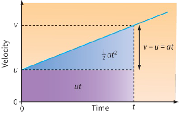
We can find the first two equations from the velocity–time graph shown in Figure 2.16. The graph represents the motion of an object. Its initial velocity is u. After time t, its final velocity is v.
Equation 1
The graph of Figure 2.16 is a straight line, therefore the object’s acceleration a is constant. The gradient (slope) of the line is equal to acceleration.
The acceleration is defined as:
$a = \frac{{(v - u)}}{t}$
which is the gradient of the line. Rearranging this gives the first equation of motion:
$v = u + at$ (equation 1)
Equation 2
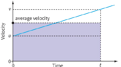
Displacement is given by the area under the velocity–time graph. Figure 2.17 shows that the object’s
average velocity is half-way between u and v. So the object’s average velocity, calculated by averaging its
initial and final velocities, is given by:
The object’s displacement is the shaded area in Figure 2.17. This is a rectangle, and so we have:
displacement = average velocity $ \times $ time taken
and hence:
$s = \frac{{(u = v)}}{2} \times t$ (equation 2)
Equation 3
From equations 1 and 2, we can derive equation 3:
$v = u + at$ (equation 1)
$s = \frac{{(u + v)}}{2} \times t$ (equation 2)
Substituting v from equation 1 gives:
$\begin{array}{l}
s = \frac{{(u + u + at)}}{2} \times t\\
= \frac{{2ut}}{2} + \frac{{a{t^2}}}{2}
\end{array}$
So
$s = ut + \frac{1}{2}a{t^2}$ (equation 3)
Looking at Figure 2.16, you can see that the two terms on the right of the equation correspond to the areas of the rectangle and the triangle that make up the area under the graph. Of course, this is the same area as the rectangle in Figure 2.17.
Equation 4
Equation 4 is also derived from equations 1 and 2:
$v = u + at$ (equation 1)
$s = \frac{{(u + v)}}{2} \times t$ (equation 2)
Substituting for time t from equation 1 gives:
$s = \frac{{(u + v)}}{2} \times \frac{{(u - v)}}{a}$
Rearranging this gives:
$\begin{array}{l}
2as = (u + v)(v - u)\\
= {v^2} - {u^2}
\end{array}$
or simply:
${v^2} = {u^2} + 2as$ (equation 4)
Investigating road traffic accidents
The police frequently have to investigate road traffic accidents. They make use of many aspects of physics, including the equations of motion. The next two questions will help you to apply what you have learned to situations where police investigators have used evidence from skid marks on the road.
Questions
12) Trials on the surface of a new road show that, when a car skids to a halt, its acceleration is $ - 7.0\,m\,{s^{ - 2}}$. Estimate the skid-to-stop distance of a car travelling at a speed limit of $ 30\,m\,{s^{ - 1}}$ (approximately $110\,km\,{h^{ - 1}}$ or $70 mph$).
13) At the scene of an accident on a country road, police find skid marks stretching for $50 m$. Tests on the road surface show that a skidding car decelerates at $ 6.5\,m\,{s^{ - 2}}$. Was the car that skidded exceeding the speed limit of $ 25\,m\,{s^{ - 1}}$ ($90\,km\,{h^{ - 1}}$) on this road?