Physics A Level
Chapter 2: Accelerated motion 2.12 Determining g
Physics A Level
Chapter 2: Accelerated motion 2.12 Determining g
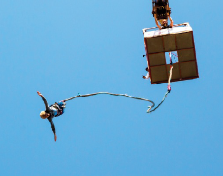
One way to measure the acceleration of free fall g would be to try bungee-jumping (Figure 2.22). You would need to carry a stopwatch, and measure the time between jumping from the platform and the moment when the elastic rope begins to slow your fall. If you knew the length of the unstretched rope, you could calculate g.
There are easier methods for finding g that can be used in the laboratory. These are described in Practical Activity 2.2.
PRACTICAL ACTIVITY 2.2: LABORATORY MEASUREMENTS OF g
Measuring g using an electronic timer
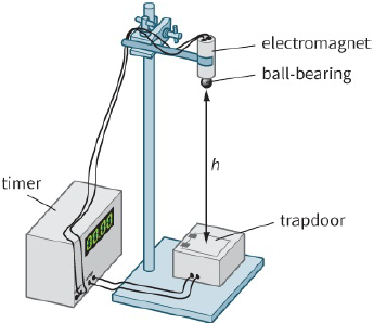
In this method, a steel ball-bearing is held by an electromagnet (Figure 2.23). When the current to the magnet is switched off, the ball begins to fall and an electronic timer starts. The ball falls through a trapdoor, and this breaks a circuit to stop the timer. This tells us the time taken for the ball to fall from rest through the distance h between the bottom of the ball and the trapdoor.
Here is how we can use one of the equations of motion to find g:
displacement $s = h$
time taken $= t$
initial velocity $u = 0$
acceleration $a = g$
Substituting in $s = ut + \frac{1}{2}a{t^2}$ gives:
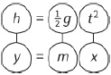
$h = \frac{1}{2}g{t^2}$
and for any values of h and t we can calculate a value for g.
A more satisfactory procedure is to take measurements of t for several different values of h. The height of the ball bearing above the trapdoor is varied systematically, and the time of fall measured several times to calculate an average for each height. Table 2.4 and Figure 2.24 show some typical results. We can deduce g from the gradient of the graph of h against ${t^2}$.
The equation for a straight line through the origin is:
$y = mx$
In our experiment we have:
| h / m | t / s | ${t^2}\,/\,{s^2}$ |
| 0.27 | 0.25 | 0.063 |
| 0.39 | 0.30 | 0.090 |
| 0.56 | 0.36 | 0.130 |
| 0.70 | 0.41 | 0.168 |
| 0.90 | 0.46 | 0.212 |
The gradient of the straight line of a graph of h against ${t^2}$ is equal to $\frac{g}{2}$.
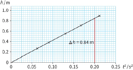
Therefore:
$\begin{array}{l}
gradient = \frac{g}{2}\\
= \frac{{0.84}}{{0.20}}\\
= 4.2\\
g = 4.2 \times 2 = 8.4\,m\,{s^{ - 2}}
\end{array}$
Sources of uncertainty
The electromagnet may retain some magnetism when it is switched off, and this may tend to slow the ball’s fall. Consequently, the time t recorded by the timer may be longer than if the ball were to fall completely freely. From $h = \frac{1}{2}g{t^2}$ , it follows that, if t is too great, the experimental value of g will be too small. This is an example of a systematic error – all the results are systematically distorted so that they are too great (or too small) as a consequence of the experimental design.
Measuring the height h is awkward. You can probably only find the value of h to within $ \pm 1mm$ at best.
So there is a random error in the value of h, and this will result in a slight scatter of the points on the graph, and a degree of uncertainty in the final value of g.
If you just have one value for h and the corresponding value for t you can use the uncertainty in h and t to find the uncertainty in g.
The percentage uncertainty in g = percentage uncertainty in $h + 2 \times $ percentage uncertainty in t.
For more about errors and combining uncertainties, see Chapter ${P_1}$.
Measuring g using a ticker-timer
Figure 2.25: shows a weight falling. As it falls, it pulls a tape through a ticker-timer. The spacing of the dots on the tape increases steadily, showing that the weight is accelerating. You can analyse the tape to
find the acceleration, as discussed in Practical Activity 2.1.
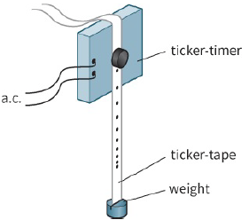
This is not a very satisfactory method of measuring g. The main problem arises from friction between the tape and the ticker-timer. This slows the fall of the weight and so its acceleration is less than g. (This is another example of a systematic error.)
The effect of friction is less of a problem for a large weight, which falls more freely. If measurements are made for increasing weights, the value of acceleration gets closer and closer to the true value of g.
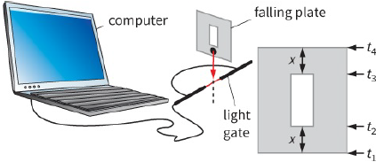
Measuring g using a light gate
Figure 2.26: shows how a weight can be attached to a card ‘interrupt’. The card is designed to break the light beam twice as the weight falls. The computer can then calculate the velocity of the weight twice as it falls, and hence find its acceleration:
$initial\,velocity\,u = \frac{x}{{{t_2} - {t_1}}}$
$final\,velocity\,v = \frac{x}{{{t_4} - {t_3}}}$
Therefore:
$acceleration\,a = \frac{{v - u}}{{{t_3} - {t_1}}}$
The weight can be dropped from different heights above the light gate. This allows you to find out whether its acceleration is the same at different points in its fall. This is an advantage over Method 1, which can only measure the acceleration from a stationary start.
Questions
18) A steel ball falls from rest through a height of $2.10 m$. An electronic timer records a time of $0.67 s$ for the fall.
a: Calculate the average acceleration of the ball as it falls.
b: Suggest reasons why the answer is not exactly $9.81\,m\,{s^{ - 2}}$.
c: Suppose the height is measured accurately but the time is measured to an uncertainty of $ \pm 0.02s$.
Calculate the percentage uncertainty in the time and the percentage uncertainty in the average acceleration. You can do this by repeating the calculation for g using a time of $0.65 s$. You can find out more about uncertainty in Chapter ${P_1}$.
19) In an experiment to determine the acceleration due to gravity, a ball was timed electronically as it fell from rest through a height h. The times t shown in Table 2.5 were obtained.
a: Plot a graph of h against ${t_1}$.
b: From the graph, determine the acceleration of free fall g.
c: Comment on your answer.
| Height h / m | 0.70 | 1.03 | 1.25 | 1.60 | 1.99 |
| Time t / s | 0.99 | 1.13 | 1.28 | 1.42 | 1.60 |
In Chapter 1, we looked at how to use a motion sensor to measure the speed and position of a moving object. Suggest how a motion sensor could be used to determine g.