CIRCUIT DESIGN

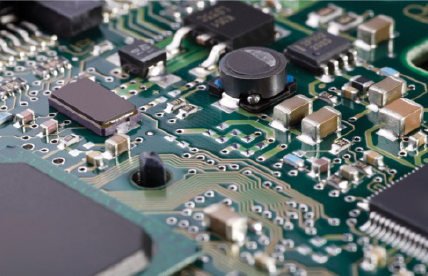
Over the years, electrical circuits have become increasingly complex, with more and more components combining to achieve very precise results (Figure 9.1). Such circuits typically include power supplies, sensing devices, potential dividers and output devices. At one time, circuit designers would start with a simple circuit and gradually modify it until the desired result was achieved. This is impossible today when circuits include many hundreds or thousands of components.
Instead, electronics engineers (Figure 9.2) rely on computer-based design software that can work out the effect of any combination of components. This is only possible because computers can be programmed with the equations that describe how current and voltage behave in a circuit. These equations, which include Ohm’s law and Kirchhoff’s two laws, were established in the $18th$ century, but they have come into their own in the $21st$ century through their use in computer-aided design (CAD) systems.

Think about other areas of industry. How have computers changed those industrial practices in the last 30 years?

You will have learnt that current may divide up where a circuit splits into two separate branches. For example, a current of $5.0 A$ may split at a junction or a point in a circuit into two separate currents of $2.0A$ and $3.0 A$. The total amount of current remains the same after it splits. We would not expect some of the current to disappear, or extra current to appear from nowhere. This is the basis of Kirchhoff’s first law, which states that the sum of the currents entering any point in a circuit is equal to the sum of the currents leaving that same point.
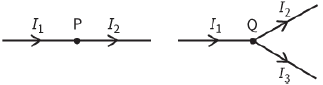
This is illustrated in Figure 9.3. In the first part, the current into point P must equal the current out, so:

${I_1}\, = \,{I_2}$

In the second part of the figure, we have one current coming into point Q, and two currents leaving. The current divides at Q. Kirchhoff’s first law gives:

${I_1}\, = \,{I_2} + {I_3}$

Kirchhoff’s first law is an expression of the conservation of charge. The idea is that the total amount of charge entering a point must exit the point. To put it another way, if a billion electrons enter a point in a circuit in a time interval of $1.0 s$, then one billion electrons must exit this point in $1.0 s$. The law can be tested by connecting ammeters at different points in a circuit where the current divides. You should recall that an ammeter must be connected in series so the current to be measured passes through it.

Questions

 

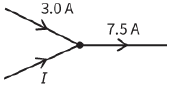
1) Use Kirchhoff’s first law to deduce the value of the current I in Figure 9.4.

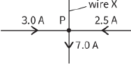
2) In Figure 9.5, calculate the current in the wire X. State the direction of this current (towards P or away from P).

Formal statement of Kirchhoff’s first law

We can write Kirchhoff’s first law as an equation:

$\Sigma {I_{in}} = \Sigma {I_{out}}$

Here, the symbol $\Sigma $ (Greek letter sigma) means ‘the sum of all’, so $\Sigma {I_{in}}$ means ‘the sum of all currents entering into a point’ and $\Sigma {I_{out}}$ means ‘the sum of all currents leaving that point’. This is the sort of equation that a computer program can use to predict the behaviour of a complex circuit.

Questions

 

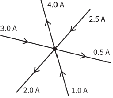
3) Calculate $\Sigma {I_{in}}$ and $\Sigma {I_{out}}$ in Figure 9.6. Is Kirchhoff’s first law satisfied?

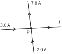
4) Use Kirchhoff’s first law to deduce the value and direction of the current I in Figure 9.7.