Chapter 10: Resistance and resistivity 10.1 The I-V characteristic for a metallic conductor
Physics A Level
Chapter 10: Resistance and resistivity 10.1 The I-V characteristic for a metallic conductor
2022-10-11
94
Crash
report
Physics (9702)
Chapter 1: Kinematics
Chapter 2: Accelerated motion
Chapter 3: Dynamics
Chapter 4: Forces
Chapter 5: Work, energy and power
Chapter 6: Momentum
Chapter 7: Matter and materials
Chapter 8: Electric current
Chapter 9: Kirchhoff’s laws
Chapter 10: Resistance and resistivity
Chapter 11: Practical circuits
Chapter 12: Waves
Chapter 13: Superposition of waves
Chapter 14: Stationary waves
Chapter 15: Atomic structure
P1 Practical skills at AS Level
Chapter 16: Circular motion
Chapter 17: Gravitational fields
Chapter 18: Oscillations
Chapter 19: Thermal physics
Chapter 20: Ideal gases
Chapter 21: Uniform electric fields
Chapter 22: Coulomb’s law
Chapter 23: Capacitance
Chapter 24: Magnetic fields and electromagnetism
Chapter 25: Motion of charged particles
Chapter 26: Electromagnetic induction
Chapter 27: Alternating currents
Chapter 28: Quantum physics
Chapter 29: Nuclear physics
Chapter 30: Medical imaging
Chapter 31: Astronomy and cosmology
P2 Practical skills at A Level
LEARNING INTENTIONS
In this chapter you will learn how to:
- state Ohm’s law
- sketch and explain the I–V characteristics for various components
- sketch the temperature characteristic for an NTC thermistor
- solve problems involving the resistivity of a material.
BEFORE YOU START
- Do you understand the terms introduced in Chapters 8 and 9: current, charge, potential difference, e.m.f., resistance and their relationships to one another?
- What are their units?
- Take turns in challenging a partner to define a term or to write down an equation linking different terms. Do not use the textbook or your notes to look up the terms.
SUPERCONDUCTIVITY
As metals are cooled, their resistance decreases. It was discovered as long ago as 1911 that when mercury was cooled using liquid helium to $4.1 K$ (4.1 degrees above absolute zero), its resistance suddenly fell to zero. This phenomenon was named superconductivity. Other metals, such as lead at $7.2 K$, also become superconductors.
When charge flows in a superconductor, it can continue in that superconductor without the need for any potential difference and without dissipating any energy. This means that large currents can occur without the unwanted heating effect that would occur in a normal metallic or semiconducting conductor.
Initially, superconductivity was only of scientific interest and had little practical use, as the liquid helium that was required to cool the superconductors is very expensive to produce. In 1986, it was discovered that particular ceramics became superconducting at much higher temperatures – above $77 K$, the boiling point of liquid nitrogen. This meant that liquid nitrogen, which is readily available, could be used to cool the superconductors and expensive liquid helium was no longer needed. Consequently, superconductor technology became a feasible proposition.
Uses of superconductors
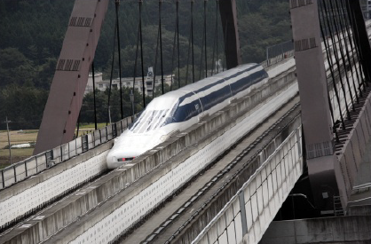
The JR-Maglev train in Japan’s Yamanashi province floats above the track using superconducting magnets (Figure 10.1). This means that not only is the heating effect of the current in the magnet coil s reduced to zero – it also means that the friction between the train and the track is eliminated and that the train can reach incredibly high speeds of up to $580\,km\,{h^{ - 1}}$.
Particle accelerators, such as the Large Hadron Collider (LHC) at the CERN research facility in Switzerland, accelerate beams of charged particles to very high energies by making them orbit around a circular track many times. The particles are kept moving in the circular path by very strong magnetic fields produced by electromagnets whose coils are made from superconductors. Much of our understanding of the fundamental nature of matter is from doing experiments in which beams of these very high speed particles are made to collide with each other.
Figure 10.1: The Japanese JR-Maglev train, capable of speeds approaching $600\,km\,{h^{ - 1}}$.
Magnetic resonance imaging (MRI) was developed in the $1940s$. It is used by doctors to examine internal organs without invasive surgery.
Superconducting magnets can be made much smaller than conventional magnets, and this has enabled the magnetic fields produced to be much more precise, resulting in better imaging.
Imagine you are a scientific consultant for a new science fiction film. You have been instructed to find a use of a superconductor to enable the hero to escape from a villain who is about to destroy the world.
What use would you come up with?
In Chapter 8, we saw how we could measure the resistance of a resistor using a voltmeter and ammeter. In this topic we are going to investigate the variation of the current – and, therefore, resistance – as the potential difference across a conductor changes.
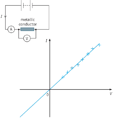
The potential difference across a metal conductor can be altered using a variable power supply or by placing a variable resistor in series with the conductor. This allows us to measure the current at different potential differences across the conductor. The results of such a series of measurements are shown graphically in Figure 10.2.
Figure 10.2: To determine the resistance of a component, you need to measure both current and
potential difference.
Look at the graph of Figure 10.2. Such a graph is known as an I–V characteristic. The points are slightly scattered, but they clearly lie on a straight line. A line of best fit has been drawn. You will see that it passes through the origin of the graph. In other words, the current I is directly proportional to the voltage V.
The straight-line graph passing through the origin shows that the resistance of the conductor remains constant. If you double the current, the voltage will also double. However, its resistance, which is the ratio of the voltage to the current, remains the same. Instead of using:
$R = \frac{V}{I}$
to determine the resistance, for a graph of I against V that is a straight line passing through the origin, you can also use:
(This will give a more accurate value for R than if you were to take a single experimental data point. Take care! You can only find resistance from the gradient if the I–V graph is a straight line through the origin.)
By reversing the connections to the resistor, the p.d. across it will be reversed (in other words, it becomes negative). The current will be in the opposite direction – it is also negative. The graph is symmetrical, showing that if a p.d. of, say, $2.0 V$ produces a current of $0.5 A$, then a p.d. of $−2.0 V$ will produce a current of $−0.5 A$. This is true for most simple metallic conductors but is not true for some electronic components, such as diodes.
You get results similar to those shown in Figure 10.2 for a commercial resistor. Resistors have different resistances, so the gradient of the I–V graph will be different for different resistors.
Question
1) Table 10.1 shows the results of an experiment to measure the resistance of a carbon resistor whose resistance is given by the manufacturer as $47\,\Omega \pm 10\% $.
a: Plot a graph to show the I–V characteristic of this resistor.
b: Do the points appear to fall on a straight line that passes through the origin of the graph?
c: Use the graph to determine the resistance of the resistor.
d: Does the value of the resistance fall within the range given by the manufacturer?