If you set up a trolley tethered between springs (Figure 18.13) you can hear the characteristic rhythm of s.h.m. as the trolley oscillates back and forth. By adjusting the mass carried by the trolley, you can achieve oscillations with a period of about two seconds.

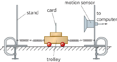
The motion sensor allows you to record how the displacement of the trolley varies with time. Ultrasonic pulses from the sensor are reflected by the card on the trolley and the reflected pulses are detected. This ‘sonar’ technique allows the sensor to determine the displacement of the trolley. A typical screen display is shown in Figure 18.14.

The motion sensor allows you to record how the displacement of the trolley varies with time. Ultrasonic pulses from the sensor are reflected by the card on the trolley and the reflected pulses are detected. This ‘sonar’ technique allows the sensor to determine the displacement of the trolley. A typical screen display is shown in Figure 18.14.

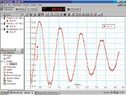
The computer can then determine the velocity of the trolley by calculating the rate of change of displacement. Similarly, it can calculate the rate of change of velocity to determine the acceleration. 
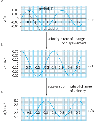
Idealised graphs of displacement, velocity and acceleration against time are shown in Figure 18.15. We will examine these graphs in sequence to see what they tell us about s.h.m. and how the three graphs are related to one another.

Displacement–time ($x–t$) graph

The displacement of the oscillating mass varies according to the smooth curve shown in Figure 18.15a.
Mathematically, this is a sine curve; its variation is described as sinusoidal. Note that this graph allows us to determine the amplitude ${x_0}$ and the period T of the oscillations. In this graph, the displacement x of the oscillation is shown as zero at the start, when t is zero. We have chosen to consider the motion to start when the mass is at the midpoint of its oscillation (equilibrium position) and is moving to the right. We could have chosen any other point in the cycle as the starting point, but it is conventional to start as shown here.

Velocity–time ($v–t$) graph

The velocity v of the oscillator at any time can be determined from the gradient of the displacement–time graph:

$v = \frac{{\Delta x}}{{\Delta t}}$

Again, we have a smooth curve (Figure 18.15b), which shows how the velocity v depends on time t. The shape of the curve is the same as for the displacement–time graph, but it starts at a different point in the cycle.
When time $t = 0$, the mass is at the equilibrium position and this is where it is moving fastest. Hence, the velocity has its maximum value at this point. Its value is positive because at time $t = 0$ it is moving towards the right.

Acceleration–time ($a–t$) graph

Finally, the acceleration a of the oscillator at any time can be determined from the gradient of the velocity–time graph:

$a = \frac{{\Delta v}}{{\Delta t}}$

This gives a third curve of the same general form (Figure 18.15c), which shows how the acceleration a depends on time t. At the start of the oscillation, the mass is at its equilibrium position. There is no resultant force acting on it so its acceleration is zero. As it moves to the right, the restoring force acts towards the left, giving it a negative acceleration. The acceleration has its greatest value when the mass is displaced farthest from the equilibrium position. Notice that the acceleration graph is ‘upside-down’ compared with the displacement graph. This shows that:

$acceleration\, \propto \, - displacement$

or

$a\, \propto \, - x$

In other words, whenever the mass has a positive displacement (to the right), its acceleration is to the left, and vice versa.