Chapter 26: Electromagnetic induction 26.3 Faraday’s law of electromagnetic induction
Physics A Level
Chapter 26: Electromagnetic induction 26.3 Faraday’s law of electromagnetic induction
2022-11-21
108
Crash
report
Physics (9702)
Chapter 1: Kinematics
Chapter 2: Accelerated motion
Chapter 3: Dynamics
Chapter 4: Forces
Chapter 5: Work, energy and power
Chapter 6: Momentum
Chapter 7: Matter and materials
Chapter 8: Electric current
Chapter 9: Kirchhoff’s laws
Chapter 10: Resistance and resistivity
Chapter 11: Practical circuits
Chapter 12: Waves
Chapter 13: Superposition of waves
Chapter 14: Stationary waves
Chapter 15: Atomic structure
P1 Practical skills at AS Level
Chapter 16: Circular motion
Chapter 17: Gravitational fields
Chapter 18: Oscillations
Chapter 19: Thermal physics
Chapter 20: Ideal gases
Chapter 21: Uniform electric fields
Chapter 22: Coulomb’s law
Chapter 23: Capacitance
Chapter 24: Magnetic fields and electromagnetism
Chapter 25: Motion of charged particles
Chapter 26: Electromagnetic induction
Chapter 27: Alternating currents
Chapter 28: Quantum physics
Chapter 29: Nuclear physics
Chapter 30: Medical imaging
Chapter 31: Astronomy and cosmology
P2 Practical skills at A Level
Earlier in this chapter, we saw that electromagnetic induction occurs when magnetic flux linking a circuit changes with time. We can now use Faraday’s law of electromagnetic induction to determine the magnitude of the induced e.m.f. in a circuit:
The magnitude of the induced e.m.f. is directly proportional to the rate of change of magnetic flux linkage.
Remember that ‘rate of change’ in physics is equivalent to ‘per unit time’. Therefore, we can write this mathematically as:
$E \propto \frac{{\Delta (N\Phi )}}{{\Delta t}}$
where $\Delta (N\Phi )$ is the change in the magnetic flux linkage in a time $\Delta t$. When working in SI units, the constant of proportionality is equal to 1. (At this level of study, you do not need to worry about why this is the case.)
Therefore:
$E = \frac{{\Delta (N\Phi )}}{{\Delta t}}$
The equation is a mathematical statement of Faraday’s law. Note that it allows us to calculate the magnitude of the induced e.m.f.; its direction is given by Lenz’s law, which is discussed later in topic 26.3 Faraday’s law of electromagnetic induction.
Now look at Worked examples 2 and 3.
WORKED EXAMPLES
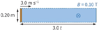
2) A straight wire of length $0.20 m$ moves at a steady speed of $3.0\,m\,{s^{ - 1}}$ at right angles to a magnetic field of flux density $0.10 T$. Use Faraday’s law to determine the magnitude of the induced e.m.f.
across the ends of the wire. Step 1: With a single conductor, $N = 1$. To determine the induced e.m.f. E, we need to find the rate of change of magnetic flux; in other words, the change in magnetic flux per unit time.
Figure 26.17: A moving wire cuts across the magnetic field
Figure 26.17 shows that in a time t, the wire travels a distance $3.0t$.
Therefore:
$\begin{array}{l}
change\,in\,magnetic\,flux\, = \,B \times change\,in\,area\\
change\,in\,magnetic\,flux\, = \,0.10 \times (3.0t \times 0.20) = 0.060t
\end{array}$ Step 2: Use Faraday’s law to determine the magnitude of the induced e.m.f.
E = rate of change of magnetic flux linkage
$E = \frac{{\Delta (N\Phi )}}{{\Delta t}}$
$\Delta \Phi = 0.06t,\,\Delta t = t$ and $N = 1$
$\begin{array}{l}
E = \frac{{0.060t}}{t}\\
= 0.060V
\end{array}$
(The t cancels. You could have done this calculation for any time t, even $1.0 s$. The results would still be the same.)
The magnitude of the induced e.m.f. across the ends of the wire is $60 mV$.
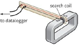
3) This example illustrates one way in which the flux density of a magnetic field can be measured, shown in Figure 26.18. A search coil is a flat-coil with many turns of very thin insulated wire.
A search coil has 2500 turns and cross-sectional area $1.2\,c{m^2}$. It is placed between the poles of a magnet so that the magnetic flux passes perpendicularly through the plane of the coil. The magnetic field between the poles has flux density $0.50 T$. The coil is pulled rapidly out of the field in a time of $0.10 s$.
Calculate the magnitude of the average induced e.m.f. across the ends of the coil.
Figure 26.18: An e.m.f. is induced in the search coil when it is moved out of the field between the poles of the magnet. A search coil can be used to detect the presence of magnetic flux
Step 1: Calculate the change in the magnetic flux linkage, $\Delta (N\Phi )$.
When the coil is pulled out from the field, the final flux linking the coil will be zero. The cross-sectional area A needs to be in ${m^2}$. Note: $1\,c{m^2} = {10^{ - 4}}\,{m^2}$.
$\begin{array}{l}
\Delta (N\Phi ) = Final\,N\Phi - inital\,N\Phi \\
\Delta (N\Phi ) = 0 - \left[ {2500 \times 1.2 \times {{10}^{ - 4}} \times 0.50} \right] = - 0.15\,Wb
\end{array}$ Step 2: Now calculate the induced e.m.f. using Faraday’s law of electromagnetic induction.
$\Delta (N\Phi ) = - 0.15\,Wb$ and $\Delta t = 0.10\,s$
$\begin{array}{l}
magnitude\,of\,e.mef\,E = \frac{{\Delta \,(N\Phi )}}{{\Delta t}}\\
= \frac{{0.15}}{{0.10}}\\
= 1.5\,V
\end{array}$
(The negative sign is not required; you only need to know the size of the e.m.f.)
Note that, in this example, we have assumed that the flux linking the coil falls steadily to zero during the time interval of $0.10 s$. The answer is, therefore, an average value of the induced e.m.f.
Questions
10) A conductor of length L moves at a steady speed v at right angles to a uniform magnetic field of flux density B.
Show that the magnitude of the induced e.m.f. E across the ends of the conductor is given by the equation: $E = BLv$
(You can use Worked example 2 to guide you through Question 10.)
11) A wire of length $10 cm$ is moved through a distance of $2.0 cm$ in a direction at right angles to its length in the space between the poles of a magnet, and perpendicular to the magnetic field. The flux density is $1.5 T$. If this takes $0.50 s$, calculate the magnitude of the average induced e.m.f. across the ends of the wire.
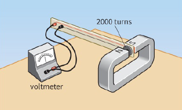
12) Figure 26.19 shows a search coil with 2000 turns and cross-sectional area $1.2\,c{m^2}$. It is placed between the poles of a strong magnet. The magnetic field is perpendicular to the plane of the coil.
The ends of the coil are connected to a voltmeter. The coil is then pulled out of the magnetic field, and the voltmeter records an average induced e.m.f. of $0.40 V$ over a time interval of $0.20 s$.
Calculate the magnetic flux density between the poles of the magnet.
Figure 26.19: Using a search coil to determine the magnetic flux density of the field between the poles of this magnet