Physics A Level
Chapter 27: Alternating currents 27.2 Alternating voltages
Physics A Level
Chapter 27: Alternating currents 27.2 Alternating voltages
Alternating current is produced in power stations by large generators like those shown in Figure 27.3.
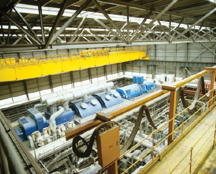
As you have already seen in Chapter 26, a generator consists of a coil rotating in a magnetic field. An e.m.f. is induced in the coil according to Faraday’s and Lenz’s laws of electromagnetic induction.
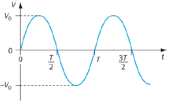
This e.m.f. V varies sinusoidally, and so we can write an equation to represent it that has the same form as the equation for alternating current:
$V = {V_0}\,\sin \omega t$
where ${V_0}$ is the peak value of the voltage. We can also represent this graphically, as shown in Figure 27.4.
Question
4) An alternating voltage V, in volt (V), is represented by the equation:
$V = 300\sin \,(100\pi t)$
a: Determine the values of ${V_0}$, $\omega $ and f for this alternating voltage.
b: Calculate V when $t = 0.002 s$. (Remember that $100\pi t$ is in radians when you calculate this.)
c: Sketch a graph to show two complete cycles of this voltage.
Measuring frequency and voltage
An oscilloscope can be used to measure the frequency and voltage of an alternating current. Practical Activity 27.1 explains how to do this. There are two types of oscilloscope. The traditional cathode-ray oscilloscope (CRO) uses an electron beam. The alternative is a digital oscilloscope, which is likely to be much more compact and which can store data and display the traces later.
PRACTICAL ACTIVITY 27.1 MEASUREMENTS USING AN OSCILLOSCOPE
A CRO is an electron beam tube, as shown in Figure 25.4, but with an extra set of parallel plates to produce a horizontal electric field at right angles to the beam (Figure 27.5).
The principles of a cathode-ray oscilloscope (CRO)
The signal into the CRO is a repetitively varying voltage. This is applied to the y-input, which deflects the beam up and down using the parallel plates ${Y_1}$ and ${Y_2}$ shown in Figure 27.5. The time-base produces a p.d. across the other set of parallel plates ${X_1}$ and ${X_2}$ to move the beam from left to right across the screen.
When the beam hits the screen of the CRO, it produces a small spot of light. If you look at the screen and slow the movement down, you can see the spot move from left to right, while the applied signal moves the spot up and down. When the spot reaches the right side of the screen, it flies back very quickly and waits for the next cycle of the signal to start before moving to the right once again. In this way, the signal is displayed as a stationary trace on the screen. There may be many controls on a CRO, even more than those shown on the CRO illustrated in Figure 27.6.
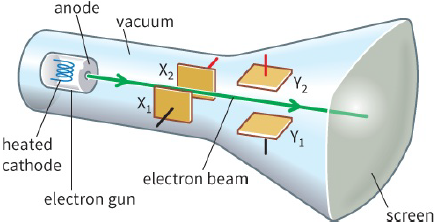
produced in the electron gun and then deflected by electric fields before they strike the screen
The controls
The X-shift and the Y-shift controls move the whole trace in the x-direction and the y-direction, respectively. The two controls that you must know about are the time-base and the Y-gain, or Ysensitivity.
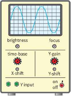
You can see in Figure 27.6 that the time-base control has units marked alongside. Let us suppose that this reads $5 ms/cm$, although it might be $5 ms/division$. This shows that $1 cm$ (or 1 division) on the xaxis represents $5 ms$. Varying the time-base control alters the speed with which the spot moves across the screen. If the time-base is changed to $1 ms/cm$, then the spot moves faster and each centimetre represents a smaller time.
The Y-gain control has a unit marked in volts/cm, or sometimes volts/division. If the actual marking is $5 V/cm$, then each centimetre on the y-axis represents $5 V$ in the applied signal.
It is important to remember that on the CRO screen, the x-axis represents time and the y-axis represents voltage.
Determining frequency and amplitude (peak value of voltage)
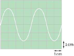
If you look at the CRO trace shown in Figure 27.7, you can see that the amplitude of the waveform, or the peak value of the voltage, is equivalent to $2 cm$ and the period of the trace is equivalent to $4 cm$.
If the Y-gain or Y-sensitivity setting is $2 V/cm$, then the peak voltage is $2 \times 2 = 4V$. If the time-base
setting is $5 ms/cm$, then the period is $4 \times 5 = 20\,ms$.
In the example:
$\begin{array}{l}
frequency = \frac{1}{{periox}}\\
= \frac{1}{{0.02}}\\
= 50\,Hz
\end{array}$
Questions
5) The Y-sensitivity and time-base settings are $5 V/cm$ and $10 ms/cm$. The trace seen on the CRO screen is the one shown in Figure 27.7.
Determine the amplitude, period and frequency of the signal applied to the Y-input of the CRO.
6) Sketch the CRO trace for a sinusoidal voltage of frequency $100 Hz$ and amplitude $10 V$, when the timebase is $10 ms/cm$ and the Y-sensitivity is $10 V/cm$.