We use mains electricity to supply us with energy. If the current and voltage are varying all the time, does this mean that the power is varying all the time too? The answer to this is yes. You may have noticed that some fluorescent lamps flicker continuously, especially if you observe them out of the corner of your eye or when you move your head quickly from one side to the other. A tungsten filament lamp would flicker too, but the frequency of the mains has been chosen so that the filament does not have time to cool down noticeably between peaks in the supply.

Root-mean-square (r.m.s.) values

There is a mathematical relationship between the peak value ${V_0}$ of the alternating voltage and a direct voltage that delivers the same average electrical power. The direct voltage is about $70\% $ of ${V_0}$. (You might have expected it to be about half, but it is more than this, because of the shape of the sine graph.) This steady direct voltage is known as the root-mean-square (r.m.s.) value of the alternating voltage. In the same way, we can think of the root-mean-square value of an alternating current, ${I_{r.m.s}}$.
The r.m.s. value of an alternating current is that steady current that delivers the same average power as the a.c. to a resistive load.
The lamps in Practical Activity 27.2 are the ‘resistive loads’. A full analysis, which we will come to shortly, shows that Ir.m.s. is related to ${I_0}$ by:

$\begin{array}{l}
{I_{r.m.s.}} = \frac{{{I_0}}}{{\sqrt 2 }}\\
 \approx 0.707 \times {I_0}
\end{array}$

This is where the factor of $70\% $ comes from. Note that this factor only applies to sinusoidal alternating currents.
We also have r.m.s. voltage ${V_{r.m.s.}}$ across the resistive load. ${V_{r.m.s.}}$ is related to the peak voltage ${V_0}$ by:

${V_{r.m.s.}} = \frac{{{V_0}}}{{\sqrt 2 }}$

PRACTICAL ACTIVITY 27.2

 

Comparing alternating current (a.c.) and direct current (d.c.)

Because the power supplied by an alternating current is varying all the time, we need to have some way of describing the average power that is being supplied. To do this, we compare an alternating current with a direct current, and try to find the direct current that supplies the same average power as the alternating current.

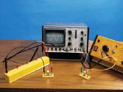
Figure 27.8 shows how this can be done in practice. Two filament lamps (our resistive loads) are placed side by side; one is connected to an a.c. supply (on the right) and the other to a d.c. supply (the batteries on the left). The a.c. supply is adjusted so that the two lamps are equally bright, indicating that the two supplies are providing energy at the same average rate. The output voltages are then compared on the double-beam oscilloscope.
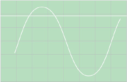
A typical trace is shown in Figure 27.9. This shows that the a.c. trace sometimes rises above the steady d.c. trace, and sometimes falls below it. This makes sense: sometimes the a.c. is delivering more power than the d.c., and sometimes less, but the average power is the same for both.

Calculating power

The importance of r.m.s. values is that they allow us to apply equations from our study of direct current to situations where the current is alternating. So, to calculate the average power dissipated in a resistor, we can use the usual formulae for power:

$P = {I^2}R = IV = \frac{{{V^2}}}{R}$

Remember that it is essential to use the r.m.s. values of I and V, as in Worked example 1. If you use peak values, your answer will be too great by a factor of 2.
Where does this factor of 2 come from? Recall that r.m.s. and peak values are related by:

${I_0} = \sqrt 2 {I_{r.m.s}}$

So, if you calculate ${I^2}R$ using ${I_0}$ instead of ${I_{r.m.s.}}$, you will introduce a factor of ${(\sqrt 2 )^2}$ or 2. The same is true if you calculate power using ${V_0}$ instead of ${V_{r.m.s.}}$. It follows that, for a sinusoidal alternating current, peak power is twice average power.

Explaining root-mean-square

We will now briefly consider the origin of the term root-mean-square and show how the factor of $\sqrt 2 $ in the equation ${I_0} = \sqrt 2 {I_{r.m.s}}$ comes about.
The equation $P = {I^2}R$ shows us that the power P is directly proportional to the square of the current I.
Figure 27.10 shows how we can calculate ${I^2}$ for an alternating current. The current I varies sinusoidally, and during half of each cycle it is negative. However, ${I^2}$ is always positive (because the square of a negative number is positive). Notice that ${I^2}$ varies up and down, and that it has twice the frequency of the current.

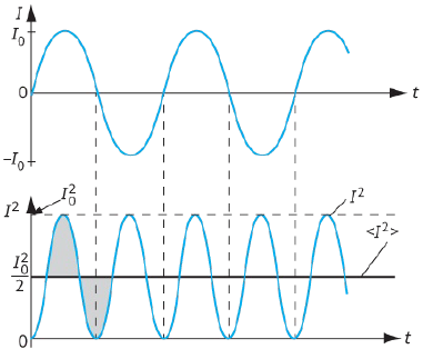
Now, if we consider $ \lt  {I^2} \gt  $, the average (mean) value of ${I^2}$, we find that its value is half of the square of the peak current (because the graph is symmetrical). That is: 

$ \lt  {I^2} \gt   = \frac{1}{2}{I_0}^2$

To find the r.m.s. value of I, we now take the square root of $ \lt  {I^2} \gt  $.
This gives:

$\begin{array}{l}
{I_{r.m.s}} = \sqrt { \lt  {I^2} \gt  }  = \sqrt {\frac{1}{2}{I_0}^2} \\
{I_0} = \sqrt 2 {I_{r.m.s}}
\end{array}$

Summarising this process: to find the r.m.s. value of the current, we find the root of the mean of the square of the current – hence r.m.s.